Contractors

Introduction

The concept of contractor is directly inspired from the ubiquituous concept of filtering algorithm in constraint programming.

Given a constraint c relating a set of variables x, an algorithm C is called a filtering algorithm if, given a box (and more generally a “domain” for x, i.e., a set of potential tuples variable can be assigned to):

\[C([x])\subseteq [x] \ \wedge \ \forall x \in [x], \ c(x) \Rightarrow x \in C([x]).\]

This relation means that:

1. Filtering gives a sub-domain of the input domain [x];

2. The resulting subdomain C([x]) contains all the feasible points with respect to the constraint c. No solution is “lost”.

This illustrated in the next picture. The constraint c (i.e., the set of points satisfying c) is represented by a green shape.

Constraint programming is the context where this concept has been formalized and intensively used. But constraint programming is by no means the only paradigm where algorithms complying with this definition have been developed. The most significant example is interval analysis, where a Newton-like iteration has been developed since the 1960’s [Moore 1966] that corresponds exactly to a filtering algorithm in the case of a constraint c of the following form:

\[c(x) \iff f(x)=0\]

where f is any (non-linear) differentiable function from \(\mathbb{R}^n\to\mathbb{R}^n\). The most famous variant of this Newton iteration is probably the Hansen-Sengupta algorithm [Hansen & Sengupta 1980].

Another important example is in picture processing, where there exist algorithms able to reduce the size of a picture to some region of interest. This kind of alorithm is today implemented in almost every digital cameras, for an automatic focus adjustment.

In this example, the constraint c is:

c(x) \(\iff\) x belongs to a region of interest

Here, it is clear that the constraint is more a consequence of the algorithm than in the other way around. This last example suggests the next definition.

An algorithm C is called a contractor if:

\[\begin{split}\begin{array}{ll} \forall [x]\in \mathbb{IR}^{n},\mathcal{C}([x])\subseteq [x] & \text{(contraction)} \\ \left(x\in [x], \mathcal{C}(\{x\})= \{x\} \right) \Rightarrow x\in \mathcal{C}([x]) & \text{(consistency)} \\ C(\{x\} )=\emptyset \Leftrightarrow \left( \exists \varepsilon >0,\forall [x]\subseteq B\left(x,\varepsilon \right) ,\mathcal{C}([x])=\emptyset \right) & \text{(continuity)} \end{array}\end{split}\]

• The first condition is the same as before.

• The second condition, the one related to the underlying constraint, has been dropped. In fact, the constraint c has been replaced by the set of insensitive points, those satisfying \(C(\{x\})=\{x\}\). So the constraint still exists, but implicitely. With this in mind, it is clear now the second condition here states again that “no solution is lost”.

• The last condition is important for some convergence issues only.

Withdrawing the link to the constraint from the definition forces one to view the contractor as a pure function:

\[C: \mathbb{IR}^n \to \mathbb{IR}^n,\]

where \(\mathbb{IR}\) denotes the set of real intervals. “Pure” means that the execution of the contractor does not depend on a context and does not produce side effects. In the former definition of filtering algorithm, the operator was depending on constraints and, in practice, constraints are external objects sharing some structures representing domains of variables. This means that the execution was depending on the context and producing side effects. This centralized architecture is often met in discrete constraint programming. It allows the implementation of many code optimization techniques, but at a price of a huge programming complexity.

In contrast, contractor programming is so simple that anyone can build a solver in a few lines. Here is the interface for contractors. As one can see, it could not be more minimalist:

class Ctc {
  public:

  // Build a contractor on nb_var variables.
  Ctc(int nb_var);

  // Performs contraction.
  // This is the only function that must be implemented in a subclass of Ctc.
  // The box in argument is contracted in-place (in-out argument).
  virtual void contract(IntervalVector& box)=0;

};

That’s all. Another advantage of removing the constraint from the definition is that it makes natural the cooperation of heterogenous contractors (would they be linked internally to a numerical constraint, a picture processing algorithm, a combinatorial problem, etc.).

The good news is that some important constraint programming techniques like propagation, shaving or constructive disjunction can actually be generalized to contractors. They don’t intrinsically need the concept of constraint.

These operators all take a set of contractors as input and produce a new (more sophisticated) contractor. The design of a solver simply amouts to the composition of such operators. All these operators form a little functionnal language, where contractors are first-class citizens. This is what is called contractor programming [Chabert & Jaulin 2009].

We present in this chapter the basic or “numerical” contractors (built from a constraint, etc.) and the operators.

Forward-Backward

Forward-backward (also known as HC4Revise) is a classical algorithm in constraint programming for contracting quickly with respect to an equality or inequality. See, e.g., [Benhamou & Granvilliers 2006], [Benhamou et al. 1999], [Collavizza 1998]. However, the more occurrences of variables in the expression of the (in)equality, the less accurate the contraction. Hence, this contractor is often used as an “atomic” contractor embedded in an higher-level operator like Propagation or Shaving.

The algorithm works in two steps. The forward step apply Interval arithmetic to each operator of the function expression, from the leaves of the expression (variable domains) upto the root node.

This is illustrated in the next picture with the constraint \((x-y)^2-z=0\) with \(x\in[0,10], \ y\in[0,4]\) and \(z\in[9,16]\):

Forward step

The backward step sets the interval associated to the root node to [0,0] (imposes constraint satisfaction) and, then, apply Backward arithmetic from the root downto the leaves:

Backward step

This contractor can either be built with a NumConstraint object or directly with a function f. In the latter case, the constraint f=0 is implicitely considered.

See examples in the tutorial.

Intersection, Union, etc.

Basic operators on contractors are :

Class name	arity	Definition
CtcIdentity	0	\([x]\mapsto[x]\)
CtcCompo	n	\([x]\mapsto(C_1\circ\ldots\circ C_n)([x])\)
CtcUnion	n	\([x]\mapsto \square C_1([x])\cup\ldots\cup C_n([x])\)
CtcFixpoint	1	\([x]\mapsto C^\infty([x])\)

Basic examples are given in the tutorial.

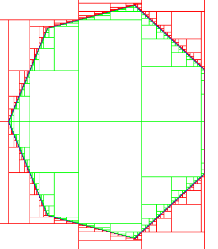
To create a union or a composition of an arbitrary number of contractors, you need first to store all the contractors references into an Array. This is illustrated in the next example where we create a contractor for the intersection of n half-spaces (delimiting a polygon) and its complementary (see the picture below where the two contractors are used to build a set).

	// Create the function corresponding to an
	// hyperplane of angle alpha
	Variable x,y,alpha;
	Function f(x,y,alpha,cos(alpha)*x+sin(alpha)*y);

	// Size of the polygon
	int n=7;

	// Array to store constraints (for cleanup)
	Array<NumConstraint> ctrs(2*n);

	// Arrays to store contractors
	Array<Ctc> ctc_out(n), ctc_in(n);

	for (int i=0; i<n; i++) {
		// create the constraints of the two half-spaces
		// delimited by f(x,y,i*2pi/n)=0
		// and store them in the array
		ctrs.set_ref(2*i,  *new NumConstraint(x,y,f(x,y,i*2*Interval::pi()/n)<=1));
		ctrs.set_ref(2*i+1,*new NumConstraint(x,y,f(x,y,i*2*Interval::pi()/n)>1));

		// create the contractors for these constraints
		// and place them in the arrays
		ctc_out.set_ref(i,*new CtcFwdBwd(ctrs[2*i]));
		ctc_in.set_ref(i, *new CtcFwdBwd(ctrs[2*i+1]));
	}

	// Composition of the "outer" contractors
	CtcCompo ctc_polygon_out(ctc_out);
	// Union of the "inner" contractors
	CtcUnion ctc_polygon_in(ctc_in);

Note: in this example, we have created constraints and contractors dynamically. We have to delete all these pointers after usage:

	// ************ cleanup ***************
	for (int i=0; i<n; i++) {
		delete &ctc_in[i];
		delete &ctc_out[i];
	}
	for (int i=0; i<2*n; i++) {
		delete &ctrs[i];
	}

Propagation

Propagation [Bessiere 2006] is another classical algorithm of constraint programming.

The basic idea is to calculate the fixpoint of a set of n contractors \(C_1\ldots,C_n\), that is:

\[(C_1\circ\ldots\circ C_n)^\infty\]

without calling a contractor when it is unecessary (as it is explained in the tutorial).

Let us first introduce for a contractor C two sets of indices: the input and output dimensions of C:

If:

\[\begin{split}\exists [x]\in\mathbb{IR}^n,\exists [y]\in\mathbb{IR}^n, \quad \forall j\!\neq\!i \ [x]_j=[y]_j \wedge \left\{\begin{array}{l} C([x])_i\neq[x]_i \vee\\ C([y])_i\neq[y]_i \vee\\ \exists j\!\neq\!i \ C([x])_j\neq C([y])_j \end{array}\right.\end{split}\]

Then i is in the input of C.

If:

\[\exists [x]\in\mathbb{IR}^n,\ C([x])_i\neq [x]_i\]

Then i is in the output of C.

Basically, input(C) contains the variables that potentially impacts the result of the contractor while ouput(C) contains the variables that are potentially impacted by the contractor.

We will explain further how this information is set in Ibex.

The propagation works as follows. It creates and maintain a set of active contractors \(\mathcal{A}\) (called “agenda”). The agenda is initialized to the full set:

\[\mathcal{A}:=\{C_1,\ldots,C_n\};\]

And the algorithm is:

1. Pop a contractor C from \(\mathcal{A}\)

2. Perform contraction: \([x]:=C([x])\).

3. If the contraction was effective, push into \(\mathcal{A}\) all the contractors C’ such that \(input(C')\cap output(C)\neq\emptyset\)

4. Return to step 1 until \(\mathcal{A}=\emptyset\).

Note: The algorithm could be improved by not pushing again in the agenda a contractor C that is idempotent (under development).

To illustrate how the propagation can be used and the benefit it provides, we compare in the next example the number of times contractors (that we chose to be forward-backward) are called in a simple fixpoint loop with the number obtained in a propagation loop.

To this aim, we need to increment a counter each time a forward-backward is called. The easiest way to do this is simply to create a subclass of CtcFwdBwd that just call the parent contraction function and increments a global counter (static variable named count).

Here is the class:

class Count : public CtcFwdBwd {
public:
	static int count;

	Count(const NumConstraint& ctr) : CtcFwdBwd(ctr) { }

	void contract(IntervalVector& box, ContractContext& context) {
		CtcFwdBwd::contract(box,context);
		count++;
	}
};

int Count::count=0;

Now, we load a set of constraints from a file. We chose on purpose a large but very sparse problem (makes propagation advantageous) and create our “counting” contractor for each constraint:

	// Load a system of constraints
	System sys(IBEX_BENCHS_DIR "/polynom/DiscreteBoundary-0100.bch");

	// The array of contractors we will use
	Array<Ctc> ctc(sys.nb_ctr);

	for (int i=0; i<sys.nb_ctr; i++)
		// Create contractors from constraints and store them in "ctc"
		ctc.set_ref(i,*new Count(sys.ctrs[i]));

Fixpoint ratio

The two contractors (CtFixPoint and CtcPropag) take also as argument a “fixpoint ratio”. The principle is that if a contraction does not remove more that

(ratio \(\times\) the diameter of a variable domain),

then this reduction is not propagated. The default value is 0.01 in the case of propagation, 0.1 in the case of fixpoint.

Warning: In theory (and sometimes in practice), the fixpoint ratio gives no information on the “distance” between the real fixpoint and the one we calculate.

Here we fix the ratio to 1e-03 for both:

	double prec=1e-03;            // Precision upto which we calculate the fixpoint

We can finally build the two strategies, call them on the same box and observe the number of calls. We also check that the final boxes are equal, up to the precision required.

With a fix point:

	// =============================== with simple fixpoint ==============================
	Count::count=0;               // initialize the counter

	CtcCompo compo(ctc);          // make the composition of all contractors
	CtcFixPoint fix(compo,prec);  // make the fixpoint

	IntervalVector box=sys.box;   // tested box (load domains written in the file)

	fix.contract(box);

	output << " Number of contractions with simple fixpoint=" << Count::count << endl;

With a propagation:

	// ================================= with propagation =================================
	Count::count=0;                            // initialize the counter

	CtcPropag propag(ctc, prec);   // Propagation of all contractors

	IntervalVector box2=sys.box;               // tested box (load domains written in the file)

	propag.contract(box2);

	output << " Number of contractions with propagation=" << Count::count << endl;

	output << " Are the results the same? " << (box.rel_distance(box2)<prec? "YES" : "NO") << endl;

The display is:

 Number of contractions with simple fixpoint=700
 Number of contractions with propagation=121
 Are the results the same? YES

Input and Output variables

The input variables (the ones that potentially impacts the contractor) and the output variables (the ones that are potentially impacted) are two lists of variables stored under the form of “bitsets”.

A biset is nothing but an (efficiently structured) list of integers.

These bitsets are the two following fields of the``Ctc`` class:

/**
 * The input variables (NULL pointer means "unspecified")
 */
BitSet* input;

/**
 * The output variables NULL pointer means "unspecified")
 */
BitSet* output;

These fields are not built by default. One reason is for allowing the distinction between an empty bitset and no bitset (information not provided). The other is that, in some applications, the number of variables is too large so that one prefers not to build these data structures even if they are very compacted.

To show the usage of these bitsets and their impact on propagation, we consider the same example as before. Let us now force the input/output bitsets of each contractors to contain every variable:

class Count2 : public CtcFwdBwd {
public:
	static int count;

	Count2(const NumConstraint& ctr) : CtcFwdBwd(ctr) {

		// The input bitset should have been created
		// by the constructor CtcFwdBwd
		assert(input!=NULL);

		// overwrite the input and output lists calculated
		// by CtcFwdBwd by adding all the variables
		for (int i=0; i<nb_var; i++) {
			input->add(i);
			output->add(i);
		}
	}

	void contract(IntervalVector& box, ContractContext& context) {
		CtcFwdBwd::contract(box,context);
		count++;
	}
};

int Count2::count=0;

We observe now that the fixpoint with CtcPropag is reached with as many iterations as without CtcPropag:

 Number of contractions with propagation=700

If you build a contractor from scratch (not inheriting a built-in contractor like we have just done), don’t forget to create the bitsets before using them with add/remove.

Here is a final example. Imagine that we have implemented a contraction algorithm for the following constraint (over 100 variables):

\[\forall i, 0\le i \le 49, \quad x[2\times i]>0 \Longrightarrow x[2\times i+1]=0.\]

The the input (resp. output) variables is the set of even (resp. odd) numbers. Here is how the initialization could be done:

class MyCtc : public Ctc {

	MyCtc() : Ctc(100) { // my contractor works on 100 variables

		// create the input list with all the variables set by default
		input = new BitSet(BitSet::all(100));
		// remove all the odd variables
		for (int i=0; i<100; i++)
			if (i%2==1) input->remove(i);

		// create the output list with all the variables unset by default
		output = new BitSet(BitSet::empty(100));
		// add all the odd variables
		for (int i=0; i<100; i++)
			if (i%2==1) output->add(i);
	}

The accumulate flag

The accumate flag is a subtle tuning parameter you may ignore on first reading.

As you know now, one annoyance with continuous variables is that we have to stop the fixpoint before it is actually reached, which means that unsignificant contractions are not propagated.

Now, to measure the significance of a contractor, we look at the intervals after contraction and compare them to the intervals just before contraction.

One little risk with this strategy is when a lot of unsignificant contractions gradually contracts domains to a point where the overall contraction has become significant. The propagation algorithm may stop despite of this significant contraction.

The accumulate flag avoids this by comparing not with the intervals just before the current contraction, but the intervals obtained after the last significant one. The drawback, however, is that all the unsignificant contractions are cumulated and attributed to the current contraction, whence a little loss of efficiency.

To set the accumulate flag, just write:

CtcPropag propag(...);
propag.accumulate = true;

Often, in practice, setting the accumulate flag results in a sligthly better contraction with a little more time.

HC4

HC4 is the classical “constraint propagation” loop that we found in the literature [Benhamou & al., 1999]. It allows to contract with respect to a system of constraints.

In Ibex, the CtcHC4 contractor is simply a direct specialization of CtcPropag (the propagation contractor).

The contractors that are propagated are nothing but the default (Forward-Backward) contractors associated to every constraint of the system.

Here is an example:

	// Load a system of equations
	System sys(IBEX_BENCHS_DIR "/others/hayes1.bch");
	// Create the HC4 propagation loop with this system
	CtcHC4 hc4(sys);

	// Test the contraction
	IntervalVector box(sys.box);
	output << " Box before HC4:" << box << endl;
	hc4.contract(box);
	output << " Box after HC4:" << box << endl;

And the result:

 Box before HC4:([-0.9000000000000001, -0.7] ; [-0.03000000000000001, -0.01] ; [-2.700000000000001, -2.6] ; [0.7, 0.8000000000000001] ; [1.35, 1.450000000000001] ; [6.9, 7] ; [1.15, 1.25])
 Box after HC4:([-0.8544702651561549, -0.776666666666666] ; [-0.03000000000000001, -0.01] ; [-2.700000000000001, -2.6] ; [0.7, 0.8000000000000001] ; [1.35, 1.450000000000001] ; [6.9, 7] ; [1.15, 1.25])

Inverse contractor

Given

• a function \(f:\mathbb{R}^n\to\mathbb{R}^m\)

• a contractor \(C:\mathbb{IR}^m\to\mathbb{IR}^m\)

The inverse of C by f is a contractor from \(\mathbb{IR}^n\to\mathbb{IR}^n\) denoted by \(f^{-1}(C)\) that satisfies:

\[\forall [x]\in\mathbb{IR}^n, \quad \Bigl(f^{-1}(C)\Bigr)[x] \supseteq \{ x \in[x], \exists y\in C(f([x])) \}.\]

To illustrate this we shall consider the function

\[t\mapsto (\cos(t),\sin(t))\]

and a contractor with respect to the constraint

\[x\ge0, y\ge 0\]

	// Build a contractor on R² wrt (x>=0 and y>=0).

	Function gx("x","y","x");   // build (x,y)->x
	Function gy("x","y","y");   // build (x,y)->y

	NumConstraint geqx(gx,GEQ); // build x>=0
	NumConstraint geqy(gy,GEQ); // build y>=0

	CtcFwdBwd cx(geqx);
	CtcFwdBwd cy(geqy);

	CtcCompo compo(cx,cy);     // final contractor wrt (x>=0, y>=0)

	// Build a mapping from R to R²
	Function f("t","(cos(t),sin(t))");

	// Build the inverse contractor
	CtcInverse inv(compo,f);

	double pi=3.14;
	IntervalVector box(1,Interval(0,2*pi));

	inv.contract(box);
	output << "contracted box (first time):" << box << endl;

	inv.contract(box);
	output << "contracted box (second time):" << box << endl;

This gives:

contracted box (first time):([0, 3.141592653589794])
contracted box (second time):([0, 1.570796326794897])

Shaving

The shaving operator consists in calling a contractor C onto sub-parts (“slices”) of the input box. If a slice is entirely eliminated by C, the input box can be contracted by removing the slice from the box.

This operator can be viewed as a generalization of the SAC algorithm in discrete domains [Bessiere and Debruyne 2004]. The concept with continuous constraint was first introduced in [Lhomme 1993] with the “3B” algorithm. In this paper, the sub-contractor C was HC4.

(to be completed)

initial box

Acid & 3BCid

(to be completed)

Polytope Hull

Consider first a system of linear inequalities. Ibex gives you the possibility to contract a box to the hull of the polytope (the set of feasible points). This is what the contractor CtcPolytopeHull stands for.

This contractor calls the linear solver Ibex has been configured with (Soplex, Cplex, CLP) to calculate for each variable \(x_i\), the following bounds:

\[\min_{A x \le b \wedge x\in[x]} \{ x_i \} \quad \mbox{and} \quad \max_{A x \le b \wedge x\in[x]} \{ x_i \}.\]

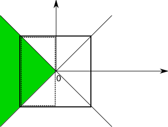
where [x] is the box to be contracted. Consider for instance

\[\begin{split}\left\{\begin{array}{l}x_1+x_2\le 0\\ x_1-x_2\le 0\\\end{array}\right.\end{split}\]

Let [x] be [-1,1]x[-1,1]. The following picture depicts the polytope (which is rather a polyhedron in this case) in green, the initial box and the result of the contraction (dashed box).

The corresponding program is:

	// build the matrix
	double _A[4]= {1,1,1,-1};
	Matrix A(2,2,_A);

	// build the vector
	Vector b=Vector::zeros(2);

	// create the linear system (with fixed matrix/vector)
	LinearizerFixed lin(A,b);

	// create the contractor w.r.t the linear system
	CtcPolytopeHull ctc(lin);

	// create a box
	IntervalVector box(2,Interval(-1,1));

	// contract it
	output << "box before contraction=" << box << endl;
	ctc.contract(box);
	output << "box after contraction=" << box << endl;

The output is:

box before contraction=([-1, 1] ; [-1, 1])
box after contraction=([-1, 0] ; [-1, 1])

In case of a non-linear system, it is also possible to call the CtcPolytopeHull contractor, providing that you give a way to linearize the non-linear system. Next section describes linearization techniques and gives an example of CtcPolytopeHull with a non-linear system.

Linearizations

Linearization procedures in Ibex are embbeded in a class inheriting the Linearizer interface.

There exists some built-in linearization techniques, namely:

• LinearizerXTaylor: a corner-based Taylor relaxation [Araya & al., 2012].

• LinearizerAffine2: a relaxation based on affine arithmetic [Ninin & Messine, 2009].

• LinearizerCompo: a combination of several techniques (the polytope is the intersection of the polytopes calculated by each technique)

• LinearizerFixed: a fixed linear system (as shown in the example above)

This Linearizer interface only imposes to implement a virtual function called linearize:

class Linearizer {
public:

     /**
      * Build a linearization procedure on nb_var variables.
      */
     Linearizer(int nb_var);

     /**
      * Add constraints in a LP solver.
      *
      * The constraints correspond to a linearization of the
      * underlying system, on the given box.
      *
      * This function must be implemented in the subclasses.
      *
      * \return the number of constraints (possibly 0) or -1 if the linear system is
      *         infeasible.
      */
     virtual int linearize(const IntervalVector& box, LinearSolver& lp_solver)=0;
};

The linearizer takes as argument a box because, most of the time, the way you linearize a nonlinear system depends on the domain of the variables. In other words, adding the 2*n bound constraints that represent the box to the system allow to build a far smaller polytope.

The second argument is the linear solver. This is only for efficiency reason: instead of building a matrix A and a vector b, the function directly enters the constraints in the linear solver. Let us now give an example.

Giving an algorithm to linearize a non-linear system is beyond the scope of this documentation so we shall here artificially linearize a linear system. The algorithm becomes trivial but this is enough to show you how to implement this interface. So let us take the same linear system as above and replace the LinearizerFixed instace by an instance of a home-made class:

/**
 * My own linear relaxation of a system
 */
class MyLinearRelax : public Linearizer {
public:
	/**
	 * We actually only accept linear systems Ax<=b :)
	 */
	MyLinearRelax(const Matrix& A, const Vector& b) : Linearizer(2), A(A), b(b) { }

	virtual int linearize(const IntervalVector & box, LPSolver& lp_solver)  {
		for (int i=0; i<A.nb_rows(); i++)
			// add the constraint in the LP solver
			lp_solver.add_constraint(A[i],LEQ,b[i]);

		// we return the number of constraints
		return A.nb_rows();
	}

	Matrix A;
	Vector b;
};

Replacing the LinearizerFixed instance by an instance of MyLinearizer gives exactly the same result.

Exists and ForAll

The CtcExist and CtcForAll contractors allow to deal with quantifiers in constraints, in a generic way.

Assume we have built a contractor C w.r.t. a constraint c(x,y) (note that we have deliberatly split here the variables of c into two sub-sets: \(x=(x_1,\ldots)\) and \(y=(y_1,\ldots)\)).

The CtcExist operator produces from C a contractor with respect to the constraint c where the variable y has been existantially quantified. More precsiely, the result is a contractor w.r.t. to the constraint c’ defined as follows:

\[c'(x) \iff \exists y\in[y], \ c(x,y).\]

where [y] is a a user-defined box.

Similarly, CtcForAll produces a contractor w.r.t.:

\[\forall y\in[y], \ c(x,y).\]

It is important to notice that the contractor CtcExist/CtcForAll expects as input two boxes, each playing a different role:

• a box that represents the domain of y. This box is read or written in a specific field of CtcExist/CtcForAll called y_init. The domain of y is a parameter that must be initialized priori to contractions. It can also be dynamically updated between two contractions but it is considered as fixed during one contraction.

• a box that represents the domain of x: this is the box that CtcExist/CtcForAll waits as a contractor. This box is the one in argument of the contract(...) function.

The contractors work as depicted on the following pictures (which illustrate the principles of the algorithms, but the actual implementation is a little more clever).

CtcExist. (a) The domain of y is split until a precision of \(\varepsilon\) is reached.

CtcExist. (b) each box is contracted with the sub-contractor and projected onto x. The result is the union (hull) of all these projections (the interval in green).

CtcForAll. (a) The domain of y is split until a precision of \(\varepsilon\) is reached. A box is then formed by taking the midpoint for y.

CtcForAll. (b) each box is contracted with the sub-contractor and projected onto x. The result is the intersection of all these projections (the interval in green).

Here is a first example. We consider the constraint \(c(x,y)\iff x^2+y^2\le 1\). When a constraint is given directly to a CtCExist/CtcForAll operator, this constraint is automatically transformed to a CtcFwdBwd contractor.

If the domain for y is set to [-1,1], the set of all x such that it exists y in [-1,1] with (x,y) satisfying the constraint is also [-1,1]. This can be observed in the following program:

	// create a constraint on (x,y)
	Variable x,y;
	NumConstraint c(x,y,sqr(x)+sqr(y)<=1);

	// create domains for x and y
	IntervalVector box_x(1, Interval(-10,10));
	IntervalVector box_y(1, Interval(-1,1));

	// set the precision that controls how much y will be bisected
	double epsilon=1.0;

	// create a contractor on x by transforming y into an
	// existentially-quantified parameter.
	CtcExist exist_y(c,y,box_y,epsilon);

	// contract the domain of x
	output << "box before contraction=" << box_x << endl;
	exist_y.contract(box_x);
	output << "box after contraction=" << box_x << endl;

The output is:

box before contraction=([-10, 10])
box after contraction=([-1, 1])

In this example, we have set the value of \(\varepsilon\) to 1.0 which is a very crude precision. In fact, the result would have been the same with an arbitrarly large precision, simply because the contraction of the full box [-10,10]x[-1,1] is optimal in this case. In other words, splitting y (i.e., using the CtcExist operator) is so far totally superfluous.

To create a more interesting example (where optimiality of a single contraction is lost) we consider two constraints:

\[x^2+y^2\le 1 \ \wedge \ x=y.\]

The set of solutions is the segment depicted in the figure below.

Now the value of \(\varepsilon\) has an impact on the accuracy of the result, as the next program illustrates:

Note: to create a conjunction of two constraints, we introduce a vector-valued function because the current

constructor of CtCExist does not accept a System (this shall be fixed in a future release). You may also consider in this situation building CtcExist directly from a contractor.

	// create a conjunction of two constraint on (x,y)
	Variable x,y;
	Function f(x,y,Return(sqr(x)+sqr(2*y-y),y-x));
	IntervalVector z(2);
	z[0]=Interval(0,1);
	z[1]=Interval::zero();
	NumConstraint c(x,y,f(x,y)=z);

	// create domains for y
	IntervalVector box_y(1, Interval(-1,1));

	// observe the result of the contraction for
	// different precision epsilon=10^{-_log}
	for (int _log=0; _log<=8; _log++) {
		// create the domain for x
		IntervalVector box_x(1, Interval(-10,10));

		// create the exist-contractor with the new precision
		CtcExist exist_y(c,y,box_y,::pow(10,-_log));

		// contract the box
		exist_y.contract(box_x);

		output << "epsilon=1e-" << _log << " box after contraction=" << box_x << endl;
	}

The output is:

epsilon=1e-0 box after contraction=([-1, 1])
epsilon=1e-1 box after contraction=([-0.7876891814830961, 0.753733646234449])
epsilon=1e-2 box after contraction=([-0.7282133915055162, 0.7125648694394637])
epsilon=1e-3 box after contraction=([-0.7078382851418078, 0.7078470747715983])
epsilon=1e-4 box after contraction=([-0.7071415397622109, 0.7071379889246125])
epsilon=1e-5 box after contraction=([-0.7071134425561116, 0.7071112646559279])
epsilon=1e-6 box after contraction=([-0.7071073875766052, 0.7071069117102449])
epsilon=1e-7 box after contraction=([-0.7071069839675348, 0.7071068778997553])
epsilon=1e-8 box after contraction=([-0.7071069839675348, 0.7071067826254732])

Warning: As we have explained, both CtcExist and CtcForAll deploy internally a search tree on the variables y until some precision \(\varepsilon\) is reached (the precision is uniform so far). The complexity of CtcExist and CtcForAll are therefore exponential in the number \(n_y\) of variables y and with potentially a ‘’big constant’’. Roughly, the complexity is in \(O\Bigl(\Bigl[\frac{max_i \ rad(y_i)}{\varepsilon}\Bigr]^{n_y}\Bigr)\). A good way to alleviate this high complexity is to use an adaptative precision. but it is anyway strongly recommended to limit the number of quantified parameters.

The generic constructor

If you want to use a specific contractor (either because forward-backward is not appropriate or because your constraint is something more exotic), you can resort to the generic constructor. This constructor simply takes a contractor C in argument instead of a constraint. There is however another slight difference. Since there is no constraint aynmore, you cannot directly specify the parameters as symbols directly: CtcExist cannot map itself these symbols to components of boxes contracted by C (remember that contractors are pure numerical functions). So you need to explicitly state the indices of variables that are transformed into parameters. This indices are given in a bitset structure. Here is a “generic variant” of the last example. Note that we take benefit of this generic constructor to give a HC4 contractor instead of a simple forward-backward, whence a slightly better contraction.

	// create a system
	Variable x,y;
	SystemFactory fac;
	fac.add_var(x);
	fac.add_var(y);
	fac.add_ctr(sqr(x)+sqr(2*y-y)<=1);
	fac.add_ctr(x=y);

	System sys(fac);

	CtcHC4 hc4(sys);

	// create domains for y
	IntervalVector box_y(1, Interval(-1,1));

	// Creates the bitset structure that indicates which
	// component are "quantified". The indices vary
	// from 0 to 1 (2 variables only). The bitset is
	// initially empty which means that, by default,
	// all the variables are parameters.
	BitSet vars(2);

	// Add "x" as variable.
	vars.add(0);

	// observe the result of the contraction for
	// different precision epsilon=10^{-_log}
	for (int _log=0; _log<=8; _log++) {
		// create the domain for x
		IntervalVector box_x(1, Interval(-10,10));

		// create the exist-contractor with the new precision
		CtcExist exist_y(hc4,vars,box_y,::pow(10,-_log));

		// contract the box
		exist_y.contract(box_x);

		output << "epsilon=1e-" << _log << " box after contraction=" << box_x << endl;
	}

The output is:

epsilon=1e-0 box after contraction=([-0.9974937185533101, 0.9237635498752691])
epsilon=1e-1 box after contraction=([-0.7105000111038531, 0.717159647201955])
epsilon=1e-2 box after contraction=([-0.7085191318530563, 0.7081440747898437])
epsilon=1e-3 box after contraction=([-0.7072537910993831, 0.7072034883921635])
epsilon=1e-4 box after contraction=([-0.7071128637729426, 0.7071156260245542])
epsilon=1e-5 box after contraction=([-0.7071077816302066, 0.707107587705308])
epsilon=1e-6 box after contraction=([-0.7071068901987889, 0.7071068546978915])
epsilon=1e-7 box after contraction=([-0.7071067909156146, 0.7071067878864685])
epsilon=1e-8 box after contraction=([-0.7071067825315514, 0.7071067817971828])

Adaptative precision

When a CtcExist contractor is embedded in a search, one naturally asks for an adptative precision. Indeed, when the domain of [x] is large, it is counter-productive to split [y] downto maximal precision. More generally, the idea of adptative precision is to dynamically set the precision \(\varepsilon\) accordingly to the size of the contracted box [x].

You may find suprising that such adptative precision is not part of the CtcExist/CtcForAll interface. This is because the adptative behavior can be easily produced thanks to the contractor paradigm. The idea is to create a contractor that wraps CtcExist and simply update the precision. Next program illustrates the concept.

class MyCtcExist : public Ctc {
public:

	/*
	 * Create MyCtcExist. The number of variables
	 * is the number of bits set to "true" in the
	 * "vars" structure; this number is obtained
	 *  via vars.size().
	 */
	MyCtcExist(Ctc& c, const BitSet& vars, const IntervalVector& box_y) :
		Ctc(vars.size()), c(c), vars(vars), box_y(box_y) { }

	void contract(IntervalVector& box_x) {
		// Create a CtcExist contractor on-the-fly
		// and set the splitting precision on y
		// to one tenth of the maximal diameter of x.
		// The box_x is then contracted
		CtcExist(c,vars,box_y,box_x.max_diam()/10).contract(box_x);
	}


	// The sub-contractor
	Ctc& c;
	// The variables indices
	const BitSet& vars;
	// The parameters domain
	const IntervalVector& box_y;
};

It suffices now to replace a CtcExist object by a MyCtcExist one.